2 Get started
In this Chapter, we will begin to learn how to create pictures of data that people, including ourselves, can look at and learn from. R and ggplot are the tools we will use. The best way to learn them is to follow along and repeatedly write code as you go. The material in this book is designed to be interactive and hands-on. If you work through it with me using the approach described below, you will end up with a book much like this one, with many code samples along side your notes, and the figures or other output produced by that code shown nearby.
I strongly encourage you to type out your code, rather than copying and pasting the examples from the text. Typing it out will help you learn it. At the beginning it may feel like tedious transcription you don’t fully understand. But it slows you down in a way that gets you used to what the syntax and structure of R is like, and is a very effective way to learn the language. It’s especially useful for ggplot, where the code for our figures will repeatedly have a very similar structure, built up piece by piece.
2.1 Work in plain text, using RMarkdown
When taking notes, and when writing your own code, you should write plain text in a text editor. Do not use Microsoft Word or some other word processor. You may be used to thinking of your final outputs (e.g. a Word file, a PDF document, presentation slides, or the tables and figures you make) as what’s “real” about your project. Instead, it’s better to think of the data and code as what’s real, together with the text you write. The idea is that all of your finished output—your figures, tables, and text, and so on—can be procedurally and reproducibly generated from code, data, and written material stored in a simple, plain-text format.
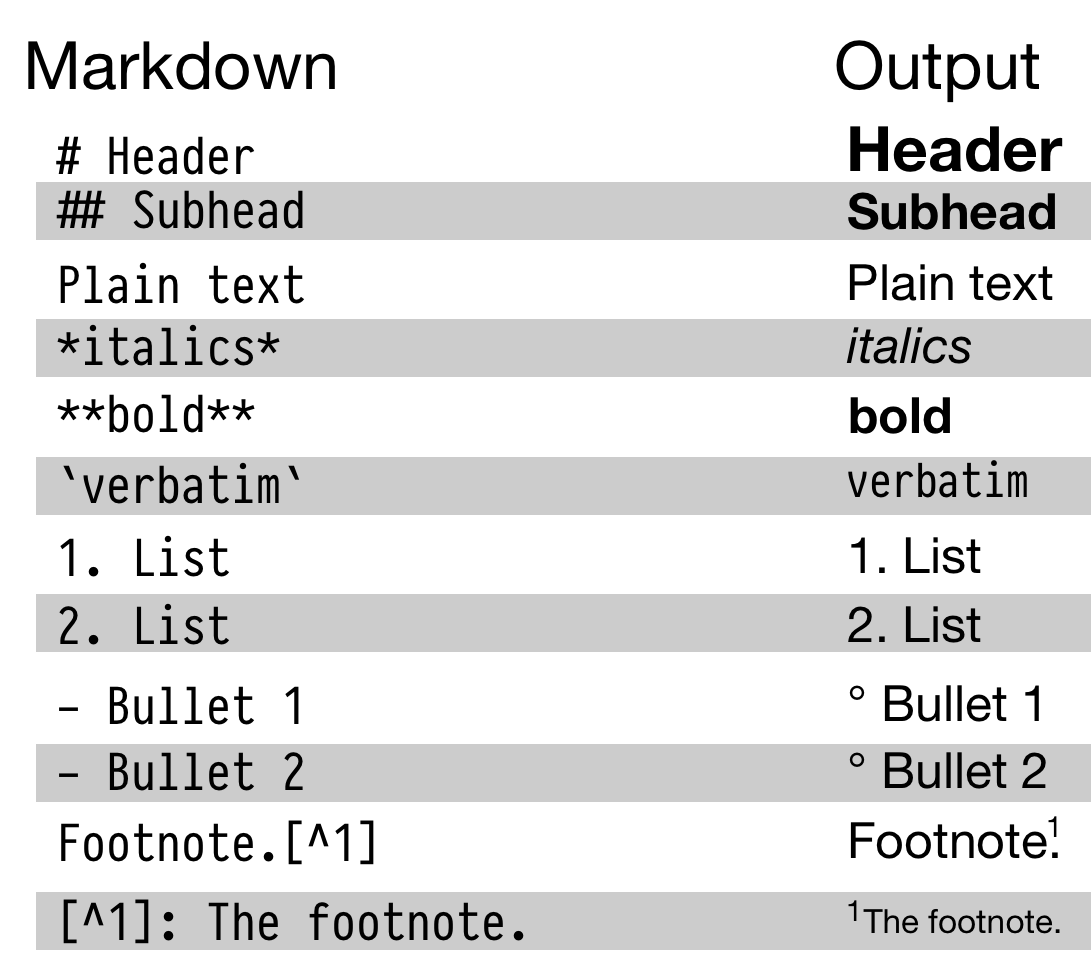
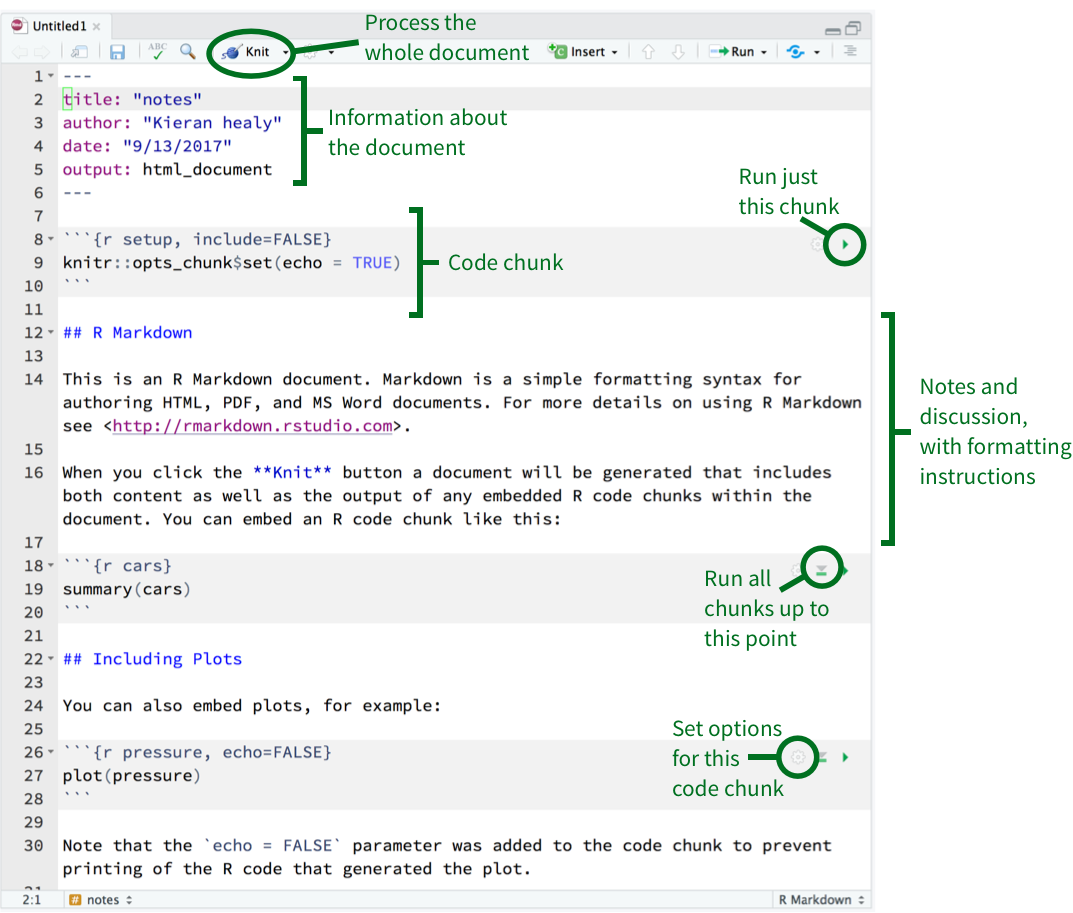
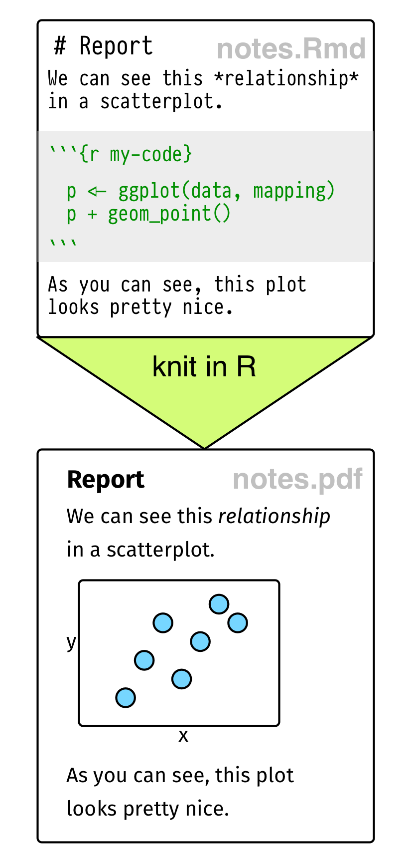 Figure 2.1: Top: Some elements of RMarkdown syntax. Bottom: From a plain text RMarkdown file to PDF output.
The ability to reproduce your work in this way is important to the scientific process. But you should also see it as a pragmatic choice that will make life easier for you in future. The reality for most of us is that the person who will most want to easily reproduce your work is you, six months or a year from now. This is especially true for graphics and figures. These often have a “finished” quality to them, as a result of much tweaking and adjustments to the details of the figure. That can make them hard to reproduce later. While it is normal for graphics to undergo a substantial amount of polishing on their way to publication, our goal is to do as much of this as possible programmatically, in code we write, rather than in a way that is retrospectively invisible, as for example when we edit an image in an application like Adobe Illustrator.
While learning ggplot, and later while doing data analysis, you will find yourself constantly pinging back and forth between three things:
- Writing code. You will write a lot of code to produce plots. You will also write code to load your data, to look quickly at tables of that data. Sometimes you will want to summarize, rearrange, subset, or augment your data, or run a statistical model with it. You will want to be able to write that code as easily and effectively as possible.
- Looking at output. Your code is a set of instructions that, when executed, produces the output you want: a table, a model, or a figure. It is often helpful to be able to see that output, and its partial results. While we’re working, it’s also useful to keep the code and the things produced by the code close together, if we can.
- Taking Notes. You will also be writing about what we are doing, and what your results mean. When learning how to do something in ggplot, for instance, you will want to make notes to yourself about what you did, why you wrote it this way rather than that, or what this new concept, function, or instruction does. Later, when doing data analysis and making figures, you will be writing up reports or drafting papers.
How can you do all this effectively? The simplest way to keep code and
notes together is to write your code and intersperse it with
comments. All programming languages have some way of demarcating lines
as comments, usually by putting a special character (like #) at the
start of the line. We could create a plain-text script file called, e.g.,
notes.r, containing code and our comments on it. This is fine as far
as it goes. But except for very short files, it will be difficult to
do anything useful with the comments we write. If we want a report
from an analysis, for example, we will have to write it up separately.
While a script file can keep comments and code together, it loses
the connection between code and its output, such as the figure we want
to produce. But there is a better alternative: we can write our notes
using RMarkdown.
An RMarkdown file is just a plain text document where text (such as notes or discussion) is interspersed with pieces, or chunks, of R code. When you feed the document to R, it knits this file into a new document by running the R code piece by piece, in sequence, and either supplementing or replacing the chunks of code with their output. The resulting file is then converted into a more easily-readable document formatted in HTML, PDF, or Word. The non-code segments of the document are plain text, but they can have simple formatting instructions in them. These are set using Markdown, a set of conventions for marking up plain text in a way that indicates how it should be formatted. The basic elements of Markdown are shown in the upper part of Figure 2.1. When you create a markdown document in R Studio, it contains some sample text to get you started.
RMarkdown documents look like the one shown schematically in the lower part of Figure 2.1. Your notes or text, with Markdown formatting as needed, are interspersed with code. There is a set format for code chunks. They look like this:
```{r}

```
Three backticks (on a U.S. keyboard, that’s the character under the escape key) followed by a pair of curly braces containing the name of the language we are using.The format is language-agnostic, and can be used with, e.g. Python and other languages. The backticks-and-braces part signal that a chunk of code is about to begin. You write your code as needed, and then end the chunk with a new line containing just three backticks.
If you keep your notes in this way, you will be able to see the code you wrote, the output it produces, and your own commentary or clarification on it in a convenient way. Moreover, you can turn it into a good-looking document right away.
2.2 Use R with RStudio
2.2.1 The RStudio environment
R itself is a relatively small application with next to no user interface.
Everything works through a command line, or console. At its most
basic, you launch it from your Terminal application (on a Mac) or
Command Prompt (on Windows) by typing R. Once launched, R awaits
your instructions at a command line of its own, denoted by the
right angle bracket symbol, >. When you type an instruction and hit
return, R interprets it and sends any resulting output back to the
console.
Figure 2.2: Bare-bones R running from the Terminal.
In addition to interacting with the console, you can also write your
code in a text file and send that to R all at once. You can use any
good text editor to write your .r scripts. But although a plain text
file and a command line is the absolute minimum you need to work with
R, it is a rather spartan arrangement. We can make life easier for
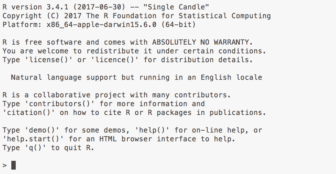
ourselves by using RStudio. RStudio is an
“integrated development environment”, or IDE. It is a separate
application from R proper. When launched, it starts up an instance of
R’s console inside of itself. It also conveniently pulls together
various other elements to help you get your work done. These include
the document where you are writing your code, the output it produces,
and R’s help system. RStudio also knows about RMarkdown, and
understands a lot about the R language and the organization of your
project. When you launch RStudio, it should look much like Figure
2.3.
Figure 2.3: The RStudio IDE.
2.2.2 Create a project
To begin, create a project. From the menu, choose File > New Project … from the
menu bar, choose the New Directory option, and create the project.You can create your new project wherever you like—most commonly it will go somewhere in your Documents folder. Once it is set up, create an RMarkdown file in the directory, with File > New File > RMarkdown.
This will give you a set of choices including the default “Document”.
The socviz library comes with a small RMarkdown template that
follows the structure of this book. To use it instead of the default
document, after selecting File > New File > RMarkdown, choose the “From
Template” option in the sidebar of the dialog box that appears. Then
choose “Data Visualization Notes” from the resulting list of options.
When the RMarkdown document appears, save it right away in your
project folder, with File > Save. The socviz template contains a
little bit of information about how RMarkdown works, together with
some headers to get you started. Read what it has to say. Look at the
code chunks and RMarkdown formatting. Experiment with knitting the
document, and compare the output to the content of the plain text
document.
RMarkdown is not required for R. An alternative is to use an R script, which just contains R commands only.You can create an r script via File > New File > R Script. R script files conventionally have the extension .r or .R. (RMarkdown files conventionally end in .Rmd.) A very brief project might just need a single .r file. But RMarkdown is very useful for documents, notes, or reports of any length, especially when you need to take notes. If you do use an .r file you can leave comments or notes to yourself by starting a line with the hash character, #. You can also add comments at the end of lines in this way, as for any particular line R will ignore whatever code or text that appears after a #.
RStudio has various keyboard and menu shortcuts to help you edit code and text quickly. For example you can insert chunks of code in your RMarkdown document with a keyboard shortcut.Command+Option+I on MacOS. Ctrl+Alt+I on Windows. This saves you from writing the backticks and braces every time. You can run the current line of code with a shortcut, too.Command+Enter on MacOS. Alt+Enter on Windows. A third shortcut gives you a pop-over display with summary of many other useful keystroke combinations.Option+Shift+K on MacOS. Alt-Shift-K on Windows. RMarkdown documents can include all kinds of other options and formatting paraphernalia, from text formatting to cross-references to bibliographical information. But never mind about those for now.
Figure 2.4: An RMarkdown file open in R Studio. The small icons in the top right-hand corner of each code chunk can be used to set options (the gear icon), run all chunks up to the current one (the downward-facing triangle), and just run the current chunk (the right-facing triangle).
To make sure you are ready to go, load the tidyverse library. The
tidyverse is a suite of related libraries for R developed by Hadley
Wickham and others. The ggplot2 library is one of its components.
The other pieces make it easier to get data in to R and manipulate it
once it is there. Either knit the notes file you created from the
socviz template, or load the library manually at the console:
library(tidyverse)

library(socviz)
We load the socviz library after the tidyverse. This library contains datasets that we will use throughout the book, along with some other tools that will make life a little easier. If you get an error message saying either library can’t be found, then re-read the “Before you Begin” section in the Preface to this book and follow the instructions there.
You only need to install a library once, but you will need to load it at the beginning of each R session with library() if you want to use the tools it contains. In practice this means that the very first lines of your working file should contain a code chunk that loads the libraries you will need in the file. If you forget to do this, then R will be unable to find the functions you want to use later on.
2.3 Things to know about R
Any new piece of software takes a bit of getting used to. This is especially true when using an IDE to work in a language like R. You are getting oriented to the language itself (what happens at the console), while learning to take notes in what might seem like an odd format (chunks of code interspersed with plain-text comments), in an IDE that that has a many features designed to make your life easier in the long run, but which can be hard to decipher at the beginning. Here are some general points to bear in mind about how R is designed. They might help you get a feel for how the language works.
2.3.1 Everything has a name
In R, everything you deal with has a name. You refer to things by
their names as you examine, use, or modify them. Named entities
include variables (like x, or y), data that you have loaded (like
my_data), and functions that you use. (More about functions
momentarily.) You will spend a lot of time talking about, creating,
referring to, and modifying things with names.
Some names are forbidden. These include reserved words like FALSE
and TRUE, core programming words like Inf, for, else, break,
function, and words for special entities like NA and NaN. (These
last two are codes designating missing data and “Not a Number”,
respectively.) You probably won’t use these names by accident, but
it’s good do know that they are not allowed.
Some names you should not use, even if they are technically permitted.
These are mostly words that are already in use for objects or
functions that form part of the core of R. These include the names of
basic functions like q() or c(), common statistical functions like
mean(), range() or var(), and built-in mathematical constants
like pi.
Names in R are case sensitive. The object my_data is not the same as
the object My_Data. When choosing names for things, be concise,
consistent, and informative. Follow the style of the tidyverse and
name things in lower case, separating words with the underscore
character, _, as needed. Do not use spaces when naming things,
including variables in your data.
2.3.2 Everything is an object
Some objects are built in to R, some are added via libraries, and some
are created by the user. But almost everything is some kind of object.
The code you write will create, manipulate, and use named objects as a
matter of course. We can start immediately. Let’s create a vector of numbers. The
command c() is a function. It’s short for “combine” or
“concatenate”. It will take a sequence of comma-separated things
inside the parentheses and join them together into a vector where each
element is still individually accessible.
c(1, 2, 3, 1, 3, 5, 25)## [1] 1 2 3 1 3 5 25Instead of sending the result to the console, we can instead assign it to an object we createYou can type the arrow using < and then -.:
my_numbers <- c(1, 2, 3, 1, 3, 5, 25)
your_numbers <- c(5, 31, 71, 1, 3, 21, 6)
To see what you made, type the name of the object and hit return:
my_numbers## [1] 1 2 3 1 3 5 25Each of our numbers is still there, and can be accessed directly if we
want. They are now just part of a new object, a vector, called
my_numbers.
You create objects by assigning them to names. The assignment
operator is <-. Think of assignment as the verb “gets”, reading
left to right. So, the bit of code above can be read as “The object
my_numbers gets the result of concatenating the following numbers:
1, 2, …” TheIf you only learn one keyboard shortcut in RStudio make it this one! Always use Option+minus on MacOS or Alt+minus on Windows to type the assignment operator. operator is two separate keys on your keyboard: the < key and the - (minus) key. Because you type this so often in R,
there is a shortcut for it in R Studio. To write the assignment
operator in one step, hold down the option key and hit -. On
Windows hold down the alt key and hit -. You will be constantly
creating objects in this way, and trying typing the two characters
separately is both tedious and prone to error. You will make
hard-to-notice mistakes like typing < - (with a space in between the
characters) instead of <-.
When you create objects by assigning things to names, they come into
existence in R’s workspace or environment. You can think of this
most straightforwardly as your project directory. Your workspace is
specific to your current project. It is the folder from which you
launched R. Unless you have particular needs (such as extremely large
datasets or analytical tastes that take a very long time) you will not
need to give any thought to where objects “really” live. Just think of
your code and data files as the permanent features of your project.
When you start up an R project, you will generally begin by loading
your data. That is, you will read it in from disk and assign it
to a named object like my_data. The rest of your code will be a series of instructions to act on and create more named objects.
2.3.3 You do things using functions
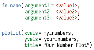 Figure 2.5: Upper: What functions look like, very schematically. Lower: an imaginary function that takes two vectors and plots them with a title. We supply the function with the particular vectors we want it to use, and the title. The vectors are objects, so are given as-is. The title is not an object, so we enclose it in quotes.
You do almost everything in R using functions. Think of a function as a special kind of object that can perform actions for you. It produces output based on the input that it receives. Like a good dog, when we want a function to do something for us, we call it. Somewhat less like a dog, it will reliably do what we tell it. We give the function some information, it acts on that information, and some results come out the other side. Functions can be recognized by the parentheses at the end of their names. This distinguishes them from other objects, such as single numbers, named vectors, tables of data, and so on.
The parentheses are what allow you to send information to the
function. Most functions accept one or more named arguments. A
function’s arguments are the things it needs to know in order to do
something. They can be some bit of your data (data = my_numbers), or
specific instructions (title = "GDP per Capita"), or an option you
want to choose (smoothing = "splines", show = FALSE). For example,
the object my_numbers is a numeric vector:
my_numbers## [1] 1 2 3 1 3 5 25But the thing we used to create it, c(), is a function. It
concatenates items into a vector composed of the series of
comma-separated elements you give it. Similarly, mean() is a
function that calculates a simple average for a vector of numbers.
What happens if we just type mean() without any arguments inside the parentheses?
mean()
# Error in mean.default() : argument "x" is missing, with no default
The error message is terse but informative. The function needs an
argument to work, and we haven’t given it one. In this case, ‘x’, the
name of another object that mean() can perform its calculation on:
mean(x = my_numbers)## [1] 5.714286mean(x = your_numbers)## [1] 19.71429While the function arguments have names that are used internally,
(here, x), you don’t strictly need to specify the name for the function to
work:
mean(my_numbers)## [1] 5.714286If you omit the name of the argument, R will just assume you are giving the function what it needs, and in a default order. The documentation for a function will tell you what the order of required arguments is for any particular function.See the Appendix for a guide to how to read the help page for a function. For simple functions that only require one or two arguments, omitting their names is usually not confusing. For more complex functions, you will typically want to use the names of the arguments rather than try to remember what the ordering is.
In general, when providing arguments to a function the syntax is
<argument> = <value>. If <value> is a named object that already
exists in your workspace, like a vector of numbers of a table of data,
then you provide it unquoted, as in mean(my_numbers). If <value>
is not an object, a number, or a logical value like TRUE, then you
usually put it in quotes, e.g., labels(x = "X Axis Label").
Functions take inputs via their arguments, do something, and return
outputs. What the output is depends on what the function does. The
c() function takes a sequence of comma-separated elements and
returns a vector consisting of those same elements. The mean()
function takes a vector of numbers and returns a single number, their
average. Functions can return far more than single numbers. The output
returned by functions can be a table of data, or a complex object such
as the results of a linear model, or the instructions needed to draw a
plot on the screen (as we shall see). They can even be other
functions. For example, the summary() function performs a series of
calculations on a vector and produces what is in effect a little table
with named elements.
A function’s argument names are internal to that function. Say you
have created an object in your environment named x, for example. A
function like mean() also has a named argument, x, but R will not
get confused by this. It will not use your x object by mistake.
As we have already seen with c() and mean(), you can assign the
result of a function to an object:
my_summary <- summary(my_numbers)When you do this, there’s no output to the console. R just puts the results into the new object, as you instructed. To look inside the object you can type its name and hit return:
my_summary## Min. 1st Qu. Median Mean 3rd Qu. Max.
## 1.00 1.50 3.00 5.71 4.00 25.002.3.4 Functions come in libraries
The code you write will be more or less complex depending on the task
you want to accomplish. Once you have gotten used to working in R, you
will probably end up writing your own functions to produce the results
that you need. But as with other programming languages, you will not
have to do everything yourself. Families of useful functions are
bundled into libraries that you can install, load into your R session,
and make use of as you work. Libraries save you from reinventing the
wheel. They make it so that you do not, for example, have to figure
out how to write code from scratch to draw a shape on screen, or load
a data file into memory. Libraries are also what allow you to build on
the efforts of others in order to do your own work. Ggplot is a
library of functions. There are many other such libraries and we will
make use of several throughout this book, either by loading them with the
library() function, or “reaching in” to them and pulling a useful
function from them directly. Writing code and functions of your own is
a good way to get a sense of the amazing volume of effort put into R
and its associated toolkits, work freely contributed by many hands
over the years and available for anyone to use.
All of the visualization we will do will involve choosing the right function or functions, and then giving those functions the right instructions through a series of named arguments. Most of the mistakes we will make, and the errors we will fix, will involve us having not picked the right function, or having not fed the function the right arguments, or having failed to provide information in a form the function can understand.
For now, just remember that you do things in R by creating and manipulating named objects. You manipulate objects by feeding information about them to functions. The functions do something useful with that information (calculate a mean, recode a variable, fit a model) and give you the results back.
table(my_numbers)## my_numbers
## 1 2 3 5 25
## 2 1 2 1 1sd(my_numbers)## [1] 8.6my_numbers * 5## [1] 5 10 15 5 15 25 125my_numbers + 1## [1] 2 3 4 2 4 6 26my_numbers + my_numbers## [1] 2 4 6 2 6 10 50The first two functions here gave us a simple table of counts and
calculated the standard deviation of my_numbers. It’s worth noticing
what R did in the last three cases. First we multiplied my_numbers
by two. R interprets that as you asking it to take each element of
my_numbers one at a time and multiply it by five. It does the same with the instruction my_numbers + 1. The single value is “recycled” down the length of the vector. By contrast, in the last case we add my_numbers to itself. Because the two objects being added are the same length, R adds each element in the first vector to the
corresponding element in the second vector. This is an example of a vectorized operation.
2.3.5 If you’re not sure what an object is, ask for its class
Every object has a class. This is the sort of object it is, whether a vector, a character string, a function, a list, and so on. Knowing an object’s class tells you a lot about what you can and can’t do with it.
class(my_numbers)## [1] "numeric"class(my_summary)## [1] "summaryDefault" "table"class(summary)## [1] "function"Certain actions you take may change an object’s class. For instance,
consider my_numbers again:
my_new_vector <- c(my_numbers, "Apple")
my_new_vector
## [1] "1" "2" "3" "1" "3" "5" "25"
## [8] "Apple"class(my_new_vector)## [1] "character"The function added the word “Apple” to our vector of numbers, as we asked. But in doing so, the result is that the new object also has a new class, switching from “numeric” to “character”. All the numbers are now enclosed in quotes. They have been turned into character strings. In that form, they can’t be used in calculations.
Most of the work we’ll be doing will not involve directly picking out this or that value from vectors or other entities. Instead we will try to work at a slightly higher level that will be easier and safer. But it’s worth knowing just the very basicsThe Appendix has a little more discussion of the basics of selecting the elements within objects. of how elements of vectors can be referred to, because the c() function in particular is a useful tool.
We will spend a lot of time in this book working with a series of datasets. These typically start life as files stored locally on your computer or somewhere remotely accessible to you. Once they are imported into R, then like everything exist as objects of some kind. R has several classes of objects used to store data. A basic one is a matrix, which consists of rows and columns of numbers. But the most common kind of data object in R is a data frame, which you can think of as a rectangular table consisting of rows (of observations) and columns (of variables). In a data frame the columns can be of different classes. Some may be character strings, some numeric, and so on. For instance, here is a very small dataset from the socviz library:
titanic## fate sex n percent
## 1 perished male 1364 62.0
## 2 perished female 126 5.7
## 3 survived male 367 16.7
## 4 survived female 344 15.6class(titanic)## [1] "data.frame"In this titanic data, two of the columns are numeric and two are not. You can access the rows and columns in various ways. For example, the $ operator allows you to pick out a named column of a data frame:
titanic$percent## [1] 62.0 5.7 16.7 15.6In Appendix A.1.2 there is a little more information about selecting particular elements from different kinds of objects.
We will also regularly encounter a slightly augmented version of a data frame called a tibble. The tidyverse libraries make extensive use of tibbles. Like data frames, they are used to store variables of different classes all together in a single table of data. They also do a little more to let us know about what they contain, and are a little more friendly when interacted with from the console. We can convert a data frame to a tibble if we want:
titanic_tb <- as_tibble(titanic)
titanic_tb
## # A tibble: 4 x 4
## fate sex n percent
## <fct> <fct> <dbl> <dbl>
## 1 perished male 1364 62.0
## 2 perished female 126 5.70
## 3 survived male 367 16.7
## 4 survived female 344 15.6Look carefully at the top and bottom of the output to see what additional information the tibble class gives you over and above the data frame version.
2.3.6 To see inside an object, ask for its structure
The str() function is sometimes useful. It lets you see what is
inside an object.
str(my_numbers)## num [1:7] 1 2 3 1 3 5 25str(my_summary)## Classes 'summaryDefault', 'table' Named num [1:6] 1 1.5 3 5.71 4 ...
## ..- attr(*, "names")= chr [1:6] "Min." "1st Qu." "Median" "Mean" ...Fair warning: while some objects are relatively simple (a vector is
just a sequence of numbers), others are more complicated, so asking
about their str() might output a forbidding amount of information to
the console. In general, complex objects are organized collections of
simpler objects, often assembled as a big list, sometimes with a
nested structure. Think for example of a master to-do list for a
complex activity like moving house. It might be organized into
sub-tasks of different kinds, several of which would themselves have
lists of individual items. One list of tasks might be related to
scheduling the moving truck, another might cover things to be donated,
and a third list of tasks might be related to setting up utilities at
the new house. In a similar sort of way, the objects we create to make
plots will have many parts and sub-parts, as the overall task of
drawing a plot has many individual to-do items. But we will be able to
build these objects up from simple forms through a series of
well-defined steps. And unlike moving house, the computer will take
care of actually carrying out the task for us. We just need to get the
to-do list right.
2.4 Be patient with R, and with yourself
Like all programming languages, R does exactly what you tell it to, rather than exactly what you want it to. This can make it frustrating to work with. It is as if one had an endlessly energetic, powerful, but also extremely literal-minded robot to order around. Remember that no-one writes fluent, error-free code on the first go all the time. From simple typos to big misunderstandings, mistakes are a standard part of the activity of programming. This is why error-checking, debugging, and testing are also a central part of programming. So, just try to be patient with yourself and with R while you use it. Expect to make errors, and don’t worry when that happens. You won’t break anything. Each time you figure out why a bit of code has gone wrong you will have learned a new thing about how the language works.
Here are three very specific things to watch out for:
- Make sure parentheses are balanced and that every opening “
(” has a corresponding closing “)”. - Make sure you complete your expressions. If you think you have completed typing your code, but instead of seeing the
>command prompt at the console you see the+character instead, that may mean R thinks you haven’t written a complete expression yet. You can hitEscorCtrl-Cto force your way back to the console and try typing your code again. - In ggplot specifically, as you will see, we will build up plots a
piece at a time by adding expressions to one another. When doing
this, make sure your
+character goes at the end of the line, and not the beginning. That is, write this:
ggplot(data = mpg, aes(x = displ, y = hwy)) +
    geom_point()
and not this:
ggplot(data = mpg, aes(x = displ, y = hwy))
+ geom_point()
R Studio will do its best to help you with the task of writing your code. It will highlight your code by syntax; it will try to match characters (like parentheses) that need to be balanced; it will try to narrow down the source of errors in code that fails to run; it will try to auto-complete the names of objects you type, so that you make fewer typos; it will make help files more easily accessible and the arguments of functions directly available. Go slowly and see how the software is trying to help you out.
2.5 Get data into R
Before we can plot anything at all we have to get our data into R in a
format it can use. Cleaning and reading in your data is one of the
least immediately satisfying pieces of an analysis, whether you use R,
StataThese are all commercial software applications for statistical analysis. Stata, in particular, is in wide use across the social sciences., SAS, SPSS, or any other statistical software. This is the reason that many of the datasets for this book are provided in a pre-prepared form via the socviz library rather than as data files you must manually
read in. However, it is something you will have to face, and that
you will want to do, sooner rather than later if you want to use the
skills you learn in this book. We might as well see how to do it now.
Even when learning R, it can be useful and very motivating to try out
the code on your own data rather than working with the sample
datasets.
Use the read_csv() function to read in comma separated data. This
function is in the readr library, one of the pieces of the
tidyverse. R and the tidyverse also have functions to import various
Stata, SAS, and SPSS formats directly. These can be found in the
haven library. All we need to do is point read_csv() at a file.
This can be a local file, e.g. in a subdirectory called data/, or it
can be a remote file. If read_csv() is given a URL or ftp address it
will follow it automatically. In this example, we have a CSV file
called organdonation.csv stored at a remote location. While online, we assign the
URL for the file to an object, for convenience, and then tell
read_csv() to fetch it for us and put it in an object named organs.
url <- "https://cdn.rawgit.com/kjhealy/viz-organdata/master/organdonation.csv"

organs <- read_csv(file = url)
## Parsed with column specification:
## cols(
## .default = col_character(),
## year = col_integer(),
## donors = col_double(),
## pop = col_integer(),
## pop.dens = col_double(),
## gdp = col_integer(),
## gdp.lag = col_integer(),
## health = col_double(),
## health.lag = col_double(),
## pubhealth = col_double(),
## roads = col_double(),
## cerebvas = col_integer(),
## assault = col_integer(),
## external = col_integer(),
## txp.pop = col_double()
## )## See spec(...) for full column specifications.The resulting message at the console tells us the read_csv() function
has assigned a class to each of the columns of the object it created
from the CSV file. There are columns with integer values, some are
character strings, and so on. (The double class is for numbers other
than integers.) Part of the reason read_csv() is telling you this
information is that it is helpful to know what class each column, or
variable, is. A variable’s class determines what sort of operations
can be performed on it. You also see this information because the
tidyverse’s read_csv() (with an underscore character in the middle
of its name) is more opinionated than an older, and also still very
widely-used function, read.csv() (with a period in the middle of its
name). The newer read_csv() will not classify variables as factors
unless you tell it to. This is in contrast to the older function,
which treats any vector of characters as a factor unless told
otherwise. Factors have some very useful features in R (especially
when it comes to representing various kinds of treatment and control
groups in experiments), but they often trip up users who are not fully
aware of them. Thus, read_csv() avoids them unless you explicitly
say otherwise.
R can read in data files in many different formats. The haven package is part of the tidyverse. It provides functions to read files created in a variety of commercial software packages.R can also talk directly to databases, a topic not covered here. If your dataset is a Stata .dta file, for instance, you can use the read_dta() function in much the same way as we used read_csv() above. This function can read and write variables stored as logical values, integers, numbers, characters and factors. Stata also has a labelled data class that the haven library partially supports.See haven’s documentation for more details. In general you will end up converting labelled variables to one of R’s basic classes. Stata also supports an extensive coding scheme for missing data. This is generally not used directly in R, where missing data is coded simply as NA. Again, you will need to take care that any labelled variables imported into R are coded properly, so that you do not end up mistakenly using missing data in your analysis.
When preparing your data for use in R, and in particular for graphing
with ggplot, bear in mind that it is best if it is represented in a
“tidy” format. Essentially this means that your data should be in
long rather than wide format, with every observation a row and
every variable a column. We will discuss this in more detail in
Chapter 3, and you can also consult the discussion of tidy data in the
Appendix.
2.6 Make your first figure
That’s enough ground-clearing for now. Writing code can be
frustrating, but it also allows you to do interesting things quickly.
Since the goal of this book is not to teach you all about R, but just
how to produce good graphics, we can postpone a lot of details until
later (or indeed ignore them indefinitely). We will start as we mean
to go on, by using a function to make a named object, and plot the
result. We will use the Gapminder dataset, which you should already
have available on your computer. We load the data with library()
and take a look.
library(gapminder)
gapminder
## # A tibble: 1,704 x 6
## country continent year lifeExp pop gdpPercap
## <fct> <fct> <int> <dbl> <int> <dbl>
## 1 Afghanistan Asia 1952 28.8 8425333 779
## 2 Afghanistan Asia 1957 30.3 9240934 821
## 3 Afghanistan Asia 1962 32.0 10267083 853
## 4 Afghanistan Asia 1967 34.0 11537966 836
## 5 Afghanistan Asia 1972 36.1 13079460 740
## 6 Afghanistan Asia 1977 38.4 14880372 786
## 7 Afghanistan Asia 1982 39.9 12881816 978
## 8 Afghanistan Asia 1987 40.8 13867957 852
## 9 Afghanistan Asia 1992 41.7 16317921 649
## 10 Afghanistan Asia 1997 41.8 22227415 635
## # ... with 1,694 more rowsThis is a table of data about a large number of countries, each observed over several years. Let’s make a scatterplot with it. Type the code below and try to get a sense of what’s happening. Don’t worry too much yet about the details.
p <- ggplot(data = gapminder,
            mapping = aes(x = gdpPercap, y = lifeExp))
p + geom_point()
Figure 2.6: Life expectancy plotted against GDP per capita for a large number of country-years.
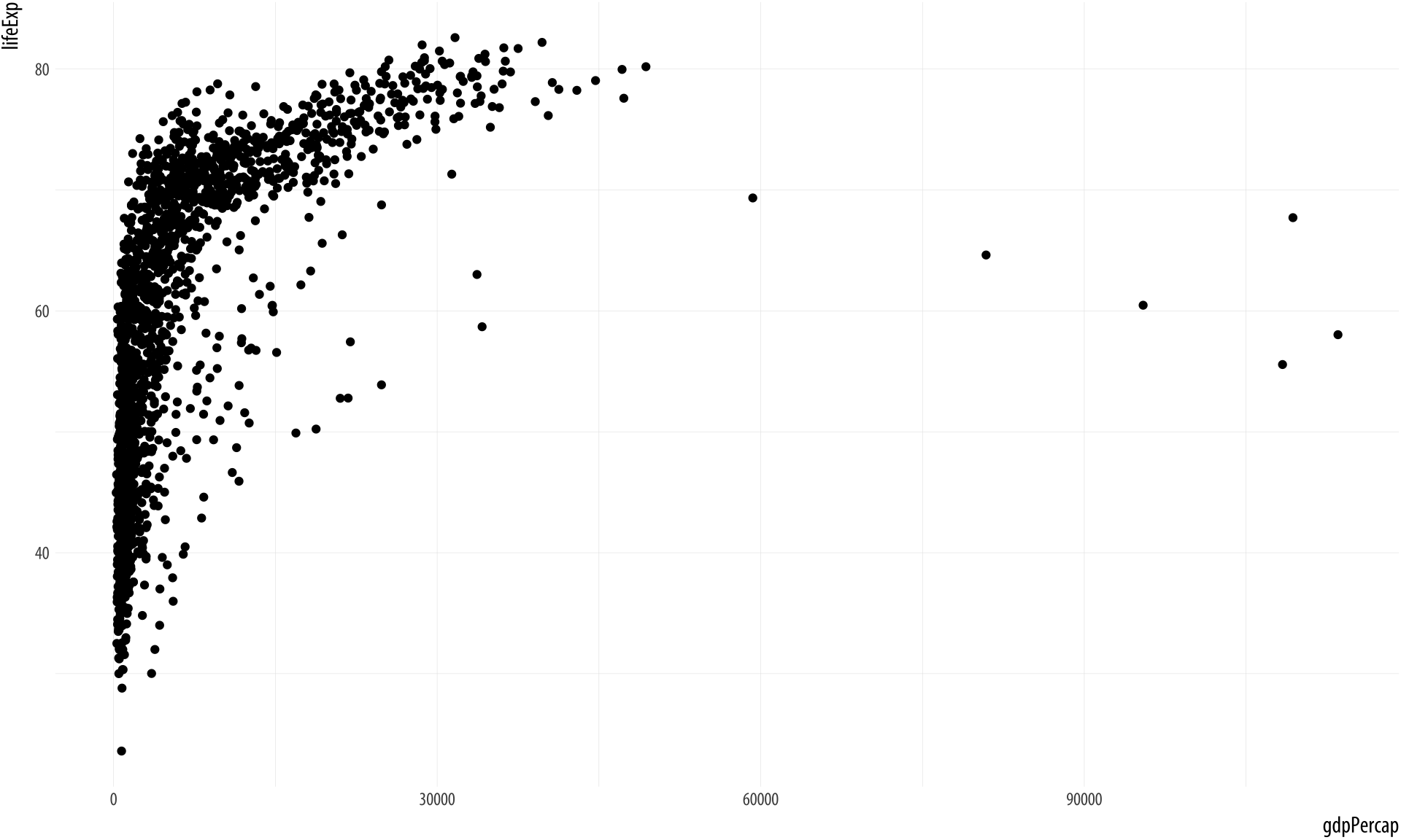
Not a bad start. Our graph is fairly legible, it has its axes informatively labeled, and it shows some sort of relationship between the two variables we have chosen. It could also be made better. Let’s learn more about how to improve it.
2.7 Where to go next
You should go straight to the next Chapter. However, you could also
spend a little more time getting familiar with R and RStudio. Some
information in the Appendix to this book might already be worth glancing
at, especially the additional introductory material on R, and the
discussion there about some common problems that tend to happen when
reading in your own data. Thereswirlstats.com are severaltryr.codeschool.com free or initially free online introductionsdatacamp.com to the R language that are worth trying. You do not need to know the material they cover in order to keep going with this book, but you might find one or more of them useful. If you get a little bogged down in any of them, or find the examples they choose are not that relevant to you, don’t worry. These introductions tend to want to introduce you to a range of programming concepts and tools that we will not need right away.
It is also worth familiarizing yourself a little with how RStudio works and with what it can do for you. The RStudio websiterstudio.com has a great deal of introductory material to help you along. You can also find a number of handy cheat sheets there that summarize different pieces of RStudio, RMarkdown, and various tidyverse packages that we will use throughout the book.rstudio.com/resources/cheatsheets These cheat-sheets are not meant to teach you the material. But they are helpful points of reference once you are up and running.